Zonal Statistics

Zonal statistics across raster & vector data can be quite computationally expensive. H3 hexagons allow performing all operations as tabular data which can be done more efficiently.

This page shows the basics of performing zonal statistics on an H3 dataset.

On H3 datasets

Here's a simple example, building on top of the previous Joining H3 datasets section:

1. Loading Elevation data as H3
2. Loading Census data as H3 (from Source Coop. Read more about it in this blogpost)
3. Joining the two datasets together
4. Calculating the zonal statistics: elevation average per census block

Since the Census data is available at H3 resolution 8, we'll use that resolution for this example

1. Loading Elevation Hex Data (copdem_elevation_hex8)

@fused.udf
def udf(
    bounds: fused.types.Bounds = [-74.556, 40.400, -73.374, 41.029],  # Default to full NYC
    res: int = 8,
):
    path = "s3://fused-asset/hex/copernicus-dem-90m/"
    
    hex_reader = fused.load("https://github.com/fusedio/udfs/tree/8024b5c/community/joris/Read_H3_dataset/")
    df = hex_reader.read_h3_dataset(path, bounds, res=res)

    return df

Returns:

hex	data_avg
613229565577683967	0.00
613229565577949183	0.00
...	...
613229775390183935	39.12
613229775390449151	0.00

2. Loading Census Data as H3 (census_h8_within_bounds)

@fused.udf
def udf(
    res: int = 8,
    bounds: fused.types.Bounds = [-74.556, 40.400, -73.374, 41.029],  # Default to full NYC
):
    common = fused.load("https://github.com/fusedio/udfs/tree/9a3aae2/public/common/")

    # Bounds to hex (to keep only hex within the current viewport)
    hex_gdf = common.bounds_to_hex(
        bounds,
        res=res,
        hex_col="hex",
    )
    hex_list = hex_gdf["hex"].tolist()

    con = common.duckdb_connect()

    qr = """
        SELECT
            state,
            county,
            POP20,
            HOUSING20,
            hex
        FROM
            's3://us-west-2.opendata.source.coop/fused/hex/release_2025_04_beta/census/2020_partitioned_h8.parquet'
        WHERE
            hex = ANY(?)
    """

    # Execute the parameterized query with hex_list directly
    df = con.execute(qr, [hex_list]).df()

    # Debug: show the resulting schema
    print(df.T)

    return df

Returns:

state	county	POP20	HOUSING20	hex
36	36005	0	0	613229520649977855
34	34023	675	225	613229784635277311

3. Joining the two datasets (elev_pop_merge)

@fused.udf
def udf(bounds: fused.types.Bounds=[-74.556, 40.4, -73.374, 41.029], res: int=8):
    
    elevation = fused.run('copdem_elevation_hex8', bounds=bounds, res=res)
    print(f"{elevation.T=}")

    population = fused.run('census_h8_within_bounds', bounds=bounds, res=res)
    print(f'{population.T=}')

    common = fused.load("https://github.com/fusedio/udfs/tree/9a3aae2/public/common/")
    con = common.duckdb_connect()

    # Joining both datasets
    qr = f"""
    SELECT 
        e.hex,
        e.data_avg as avg_elevation,
        p.POP20 as POP20,
        p.HOUSING20 as HOUSING20,
        p.county as county
    FROM elevation as e
    LEFT JOIN population as p
    ON e.hex = p.hex
    """
    join_df = con.execute(qr).df()
    
    return join_df

Returns:

hex	avg_elevation	POP20	HOUSING20	county
613229520649977855	0.215818	0	0	36005
613229784635277311	8.421718	675	225	34023
613229531395784703	0.0	NA	NA	None

4. Aggregating the elevation per census block:

@fused.udf
def udf(bounds: fused.types.Bounds=[-74.556, 40.4, -73.374, 41.029], res: int=8):
    joined = fused.run('elev_pop_merge', bounds=bounds, res=res) 

    print(joined.T)

    # Aggregate per county
    county_agg = joined.groupby(['county']).agg({
        'POP20': 'sum',
        'HOUSING20': 'sum',
        'avg_elevation': 'mean',
        'hex': 'nunique'
    }).rename(columns={'hex': 'nb_unique_hex'}).reset_index()
    
    # Calculate population density and housing units per person
    county_agg['pop_density'] = county_agg['POP20'] / county_agg['nb_unique_hex']
    county_agg['housing_per_person'] = county_agg['HOUSING20'] / county_agg['POP20']

    print(county_agg.T)
    
    return county_agg

Returns data aggregated per county:

county	POP20	HOUSING20	avg_elevation	nb_unique_hex	pop_density	housing_per_person
09001	24,374	10,216	2.575496	220	110.790909	0.419135
34003	872,587	336,021	43.332292	732	1,192.058743	0.385086
36103	195,048	68,965	24.692900	447	436.348993	0.353580
36119	622,800	242,782	39.847842	470	1,325.106383	0.389823

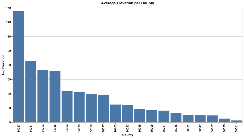
It's simple to then visualize the average elevation as a graph:

Graph: Average Elevation per County (county_avg_elevation_chart)

@fused.udf
def udf(bounds: fused.types.Bounds=[-74.556, 40.4, -73.374, 41.029], res: int=8):
    import altair as alt
    # Load data
    zonal_stats = fused.run('county_pop_housing', bounds=bounds, res=res)
    print(zonal_stats.T)
    # Prepare data for chart
    df_plot = zonal_stats[['county', 'avg_elevation']].copy()
    # Ensure county is string for axis
    df_plot['county'] = df_plot['county'].astype(str)
    chart = alt.Chart(df_plot).mark_bar().encode(
        x=alt.X('county:N', sort='-y', title='County'),
        y=alt.Y('avg_elevation:Q', title='Avg Elevation'),
        tooltip=['county', 'avg_elevation']
    ).properties(
        width=800,
        height=400,
        title='Average Elevation per County'
    )
    # Return as HTML
    return chart.to_html()

What about vector data?

In most cases, the data we want to analyze is in vector format (building footprints, census blocks, zip codes, etc.). The steps are simply:

• Transform the vector data into an H3 dataset (more info in this section)
• Follow the same steps as in the previous section